Filament Tutorial
Welcome to Filament, a humanist programming language. Computers are amazing. They can calculate incredible things super fast. They can answer questions and draw graphics. However, computers are actually very dumb. All they do is simple arithmetic. What makes them amazing is that they can do it super duper fast . To do smart things humans have to teach them. This is called programming. Anyone can program, including you!
Arithmetic
Filament understands arithmetic. Try typing in a math question like 2+2 then press the 'run'
button (or type control-return on your keyboard). Filament will show you the answer: 4 .
Now try dividing 4 by 2 or multiplying 3 by 5. Type in 4/2 . Run it. Then type 3 * 5 .
Filament uses / to mean division and * for multiplication.
Filament understands longer math equations too. For example, imagine you have a refrigerator box that is 7 feet tall by 4 feet wide by 4 feet deep. You could find out the volume of the box by multiplying all of the sides.
7 * 4 * 4
112
Units
In the above problem only we know that the 7 meant 7 feet . The computer doesn't
know because we didn't tell it. Fortunately Filament lets us tell the computer exactly what
units we mean. Let's try that again with units:
7feet * 4feet * 4feet
112 foot
Now we get 112 cuft . Cool. Filament knows to convert the answer into cubic feet.
But what if we didn't want cubic feet. We are talking about volume and there are
several different units that could represent volume. Let's ask Filament to convert it into
gallons instead.
7ft * 4ft * 4ft as gal
837.815 gallon
which gives us the answer 837.81 gallons .
Notice that this time we abbreviated feet to ft and gal for gallons .
Filament understands the full names and abbrevations for over a hundred kinds of units,
and it can convert between any of them. Here's a few more examples to try.
Convert your height into centimeters. I'm 5 foot four inches so
5feet + 4inches as cm
162.560 centimeter
Some kitchen math:
2cups + 4tablespoons
36 tablespoon
Calculate your age in seconds.
today() - date(month : 1, day : 15, year : 2003) as seconds
570585600 second
If you try to convert something that can't be converted, like area to volume, then Filament will let you know. Try this:
7ft * 4ft as gal
209.454 gallon
results in
Error. Cannot convert ft^2 to gallons.
Units are very important. They help make sure our calculations are correct. Even professionals get this wrong some times. NASA once lost a space probe worth over 100 million dollars because the software didn't convert correctly between imperial and metric units.
Superman
Now lets try a more complex problem. In one of the Superman movies he flies so fast that the world turns backwards and reverses time. That got me thinking. Is that realistic? The earth is pretty big. How long would it really take him to fly around the world?
We need some information first. How fast can Superman fly? Apparently the comics are pretty vague about his speed. Some say it's faster than light, some say it's infinite, some say it's just slighly slower than The Flash. Since this is about the real world let's go with an older claim, that Superman is faster than a speeding bullet . According to the internet, the fastest bullet ever made was was the .220 Swift which can regularly exceed 4,000 feet per second. The fastest recorded shot was at 4,665 ft/s , so we'll go with that.
Now wee need to know how big the earth is. The earth isn't perfectly spherical and of
course it would depend on exactly which part of the earth superman flew, but according to Wikipedia the
average (mean) radius of the Earth is 6,371.0 kilometers. We also know the circumference of a circle
is 2 * pi * radius . So the equation is
(6371.0km * pi * 2) / 4000ft/s as hours
Pretty fast. He could almost go three times around the earth in a single 24 hour day. But not as fast as the movie said.
Programming is both fun and useful. We can instruct computers to help us answer all sorts of interesting questions. In the next section we'll learn about groups of numbers called lists, and how to do interesting math with them.
Lists
Now let's take a look at lists. Imagine you want to add up some numbers. You could do it by adding each number separately like this:
4 + 5 + 6 + 7 + 8
30
or you could make them a list and use the sum function.
sum([4,5,6,7,8])
30
Sum is a built in function that will add all of the items in a list. There are a lot of other cool functions that work on lists. You can sort a list
sort([8,4,7,1])
1, 4, 7, 8
get the length
length([8,4,7,1])
4
or combine sum and length to find the average
nums << [8,4,7,1] sum(nums) / length(nums)
5
Making Lists
Sometimes you need to generate a list. Suppose you wanted to know the sum of every number from 0 to 100.
Of course you could write out the numbers directly, but Filament has a way to generate lists for you. It's called range .
range(10) sum(range(100))
4950
Range is flexible. You can give it both a start and end number, or even jump by steps.
range(min : 20, max : 30)
20, 21, 22, 23, 24, 25, 26, 27, 28, 29
range(100, step : 10)
0, 10, 20, 30, 40, 50, 60, 70, 80, 90
Remember that range will start at the minmum and go to one less than the max. So 0 to 10 will go up to 9.
Filament can handle big lists. If you ask for range(0,10_000_000) it will show the the first few and then ... before the last few.
range(10000)
[0, 1, 2, 3, 4, 5, 6, 7, 8, 9, 10, 11, 12, 13, 14, 15, 16, 17, 18, 19, 20, 21, 22, 23, 24 ... 9975, 9976, 9977, 9978, 9979, 9980, 9981, 9982, 9983, 9984, 9985, 9986, 9987, 9988, 9989, 9990, 9991, 9992, 9993, 9994, 9995, 9996, 9997, 9998, 9999]
Lists are very useful for lots of things, but sometimes you get more numbers than you need. Suppose you wanted all the numbers from from 0 to 20 minus the first three. Use take(list,3). Want just the last three use take(list,-3)
list << range(10) take(list, 3)
0, 1, 2
list << range(10) take(list, -3)
7, 8, 9
You can also remove items from a list with drop
drop(range(10), 8)
8, 9
And finally you can join two lists together
join([4,2], [8,6])
4, 2, 8, 6
In addition to holding data, lists let you do things that you could do on a single number, but in bulk. You can add a single number to a list
1 + [1,2,3]
2, 3, 4
or add two lists together
[1,2,3] + [4,5,6]
5, 7, 9
Math with Lists
It might seem strange to do math on lists but it's actually quite useful. Image you had a list of prices and you would like to offer a 20% discount. You can do that with a single multiplication.
prices << [4.86,5.23,10.99,8.43] sale_prices << 0.8 * prices
3.888, 4.184, 8.792, 6.744
Suppose you sold lemonade on four weekends in april, and another four in july. It would be nice to compare the sales for the different weekends to see if july did better thanks to warmer weather. You can do this by just subtracting two lists.
april << [34,44,56,42] july << [67,45,77,98] july - april
33, 1, 21, 56
Doing math with lists is also great for working with vectors. You can add them, multiply as the dot product, and calculate the magnitude.
V1 << [0,0,5] V2 << [1,0,1] V1 + V2 V1 * V2 sqrt(sum(power(V1, 2)))
5
Filtering and Mapping Lists
Lists let you search for data too. You can find items using select and a small function. Let's find all of the prime numbers up to 10000
select(range(100), where : is_prime)
2, 3, 5, 7, 11, 13, 17, 19, 23, 29, 31, 37, 41, 43, 47, 53, 59, 61, 67, 71, 73, 79, 83, 89, 97
or all numbers evenly divisible by 5
def div5 ( x : ? ) { x mod5 =0 } select(range(100), where : div5)
0, 5, 10, 15, 20, 25, 30, 35, 40, 45, 50, 55, 60, 65, 70, 75, 80, 85, 90, 95
And one of the best parts about lists is that they can hold more than numbers. You can work with lists of strings, numbers, booleans. Consider this simple list of people.
friends << ["Bart","homer","Ned"]
"Bart", "homer", "Ned"
or a list of booleans
[true,false,true]
true, false, true
Drawing Data
Bar Charts
One of the coolest things about lists is that you can draw them.
Just send a list into the chart function to see it as a bar chart.
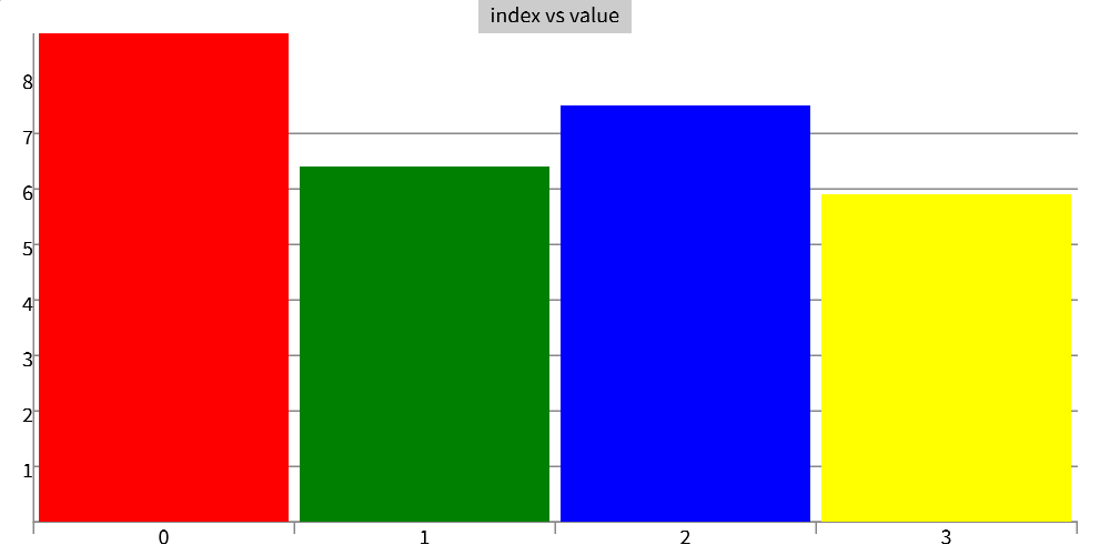
Suppose you had a list of heights of your friends.
chart([88,64,75,59])
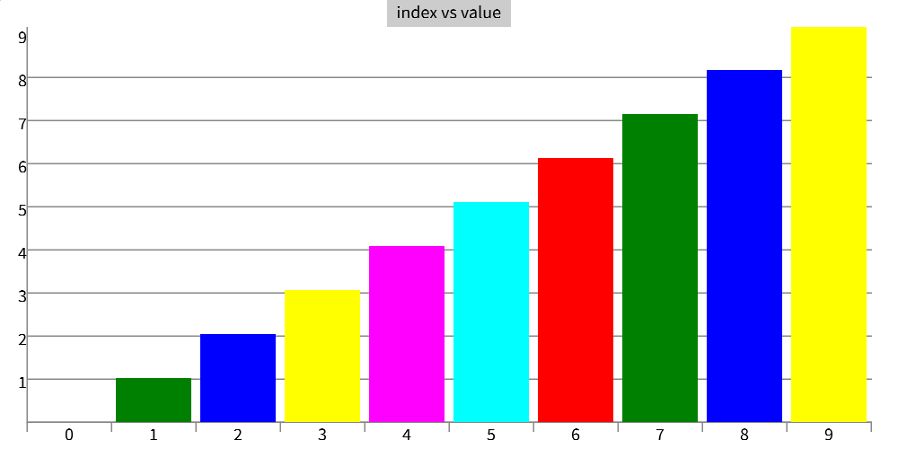
or just want to draw the numbers from 0 to 9.
chart(range(10))
Plotting equations
While you could use range , map , and chart to draw pictures of
x , power(x,2) , sin() or other math equations, there is a much
better way: using the plot function.
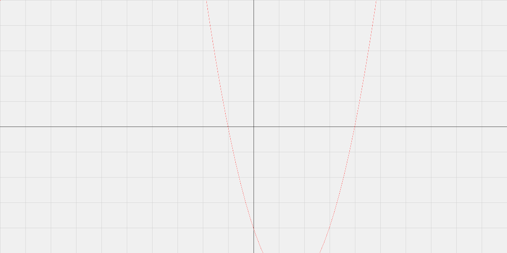
A quadratic equation
plot(y : (x)->{(x ** 2 - 3 * x - 4)})
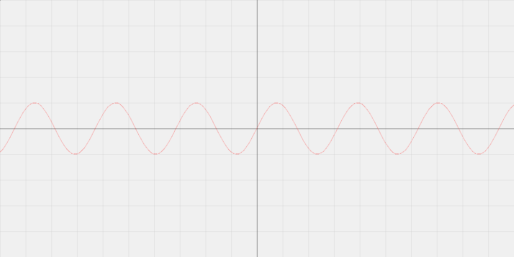
Sine wave
plot(y : theta->sin(theta * 2))
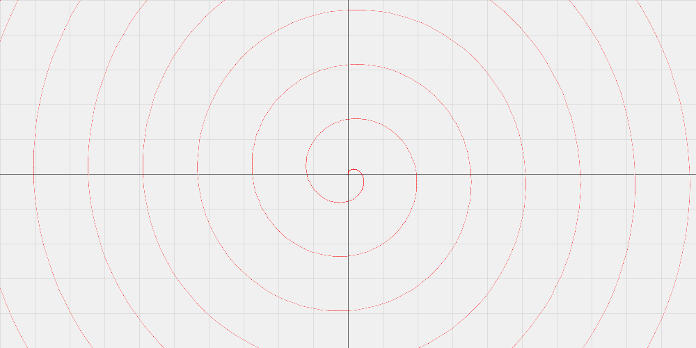
A polar Archimedes spiral
spiral << theta->0.25 * theta plot(polar : spiral, min : 0, max : pi * 32)
Charts Datasets
Even better than pulling in your own data, is working with curated datasets that have already been assembled. Filament comes with datasets for
When you load a dataset it will be shown as a table.
elements << dataset("elements")
| name | number | weight | symbol | discovered_by | discovery_date | provenance |
|---|---|---|---|---|---|---|
| Hydrogen | 1 | 1.008 | H | Henry Cavendish | January 1, 1766 | https://en.wikipedia.org/wiki/Hydrogen |
| Helium | 2 | 4.0026022 | He | Pierre Janssen | August 18, 1868 | https://en.wikipedia.org/wiki/Helium |
| Lithium | 3 | 6.94 | Li | Johan August Arfwedson | January 1, 1800 | https://en.wikipedia.org/wiki/Lithium |
| Beryllium | 4 | 9.01218315 | Be | Louis Nicolas Vauquelin | January 1, 1798 | https://en.wikipedia.org/wiki/Beryllium |
| Boron | 5 | 10.81 | B | Joseph Louis Gay-Lussac | January 1, 1808 | https://en.wikipedia.org/wiki/Boron |
| Carbon | 6 | 12.011 | C | Ancient Egypt | January 1, 2500 | https://en.wikipedia.org/wiki/Carbon |
| Nitrogen | 7 | 14.007 | N | Daniel Rutherford | January 1, 1772 | https://en.wikipedia.org/wiki/Nitrogen |
| Oxygen | 8 | 15.999 | O | Carl Wilhelm Scheele | January 1, 1771 | https://en.wikipedia.org/wiki/Oxygen |
| Fluorine | 9 | 18.9984031636 | F | André-Marie Ampère | August 26, 1812 | https://en.wikipedia.org/wiki/Fluorine |
| Neon | 10 | 20.17976 | Ne | Morris Travers | https://en.wikipedia.org/wiki/Neon | |
| Sodium | 11 | 22.989769282 | Na | Humphry Davy | https://en.wikipedia.org/wiki/Sodium | |
| Magnesium | 12 | 24.305 | Mg | Joseph Black | https://en.wikipedia.org/wiki/Magnesium | |
| Aluminium | 13 | 26.98153857 | Al | null | https://en.wikipedia.org/wiki/Aluminium | |
| Silicon | 14 | 28.085 | Si | Jöns Jacob Berzelius | https://en.wikipedia.org/wiki/Silicon | |
| Phosphorus | 15 | 30.9737619985 | P | Hennig Brand | https://en.wikipedia.org/wiki/Phosphorus | |
| Sulfur | 16 | 32.06 | S | Ancient china | https://en.wikipedia.org/wiki/Sulfur | |
| Chlorine | 17 | 35.45 | Cl | Carl Wilhelm Scheele | https://en.wikipedia.org/wiki/Chlorine | |
| Argon | 18 | 39.9481 | Ar | Lord Rayleigh | https://en.wikipedia.org/wiki/Argon | |
| Potassium | 19 | 39.09831 | K | Humphry Davy | https://en.wikipedia.org/wiki/Potassium | |
| Calcium | 20 | 40.0784 | Ca | Humphry Davy | https://en.wikipedia.org/wiki/Calcium | |
| Scandium | 21 | 44.9559085 | Sc | Lars Fredrik Nilson | https://en.wikipedia.org/wiki/Scandium | |
| Titanium | 22 | 47.8671 | Ti | William Gregor | https://en.wikipedia.org/wiki/Titanium | |
| Vanadium | 23 | 50.94151 | V | Andrés Manuel del Río | https://en.wikipedia.org/wiki/Vanadium | |
| Chromium | 24 | 51.99616 | Cr | Louis Nicolas Vauquelin | https://en.wikipedia.org/wiki/Chromium | |
| Manganese | 25 | 54.9380443 | Mn | Torbern Olof Bergman | https://en.wikipedia.org/wiki/Manganese | |
| Iron | 26 | 55.8452 | Fe | 5000 BC | https://en.wikipedia.org/wiki/Iron | |
| Cobalt | 27 | 58.9331944 | Co | Georg Brandt | https://en.wikipedia.org/wiki/Cobalt | |
| Nickel | 28 | 58.69344 | Ni | Axel Fredrik Cronstedt | https://en.wikipedia.org/wiki/Nickel | |
| Copper | 29 | 63.5463 | Cu | Middle East | https://en.wikipedia.org/wiki/Copper | |
| Zinc | 30 | 65.382 | Zn | India | https://en.wikipedia.org/wiki/Zinc | |
| Gallium | 31 | 69.7231 | Ga | Lecoq de Boisbaudran | https://en.wikipedia.org/wiki/Gallium | |
| Germanium | 32 | 72.6308 | Ge | Clemens Winkler | https://en.wikipedia.org/wiki/Germanium | |
| Arsenic | 33 | 74.9215956 | As | Bronze Age | https://en.wikipedia.org/wiki/Arsenic | |
| Selenium | 34 | 78.9718 | Se | Jöns Jakob Berzelius | https://en.wikipedia.org/wiki/Selenium | |
| Bromine | 35 | 79.904 | Br | Antoine Jérôme Balard | https://en.wikipedia.org/wiki/Bromine | |
| Krypton | 36 | 83.7982 | Kr | William Ramsay | https://en.wikipedia.org/wiki/Krypton | |
| Rubidium | 37 | 85.46783 | Rb | Robert Bunsen | https://en.wikipedia.org/wiki/Rubidium | |
| Strontium | 38 | 87.621 | Sr | William Cruickshank (chemist) | https://en.wikipedia.org/wiki/Strontium | |
| Yttrium | 39 | 88.905842 | Y | Johan Gadolin | https://en.wikipedia.org/wiki/Yttrium | |
| Zirconium | 40 | 91.2242 | Zr | Martin Heinrich Klaproth | https://en.wikipedia.org/wiki/Zirconium | |
| Niobium | 41 | 92.906372 | Nb | Charles Hatchett | https://en.wikipedia.org/wiki/Niobium | |
| Molybdenum | 42 | 95.951 | Mo | Carl Wilhelm Scheele | https://en.wikipedia.org/wiki/Molybdenum | |
| Technetium | 43 | 98 | Tc | Emilio Segrè | https://en.wikipedia.org/wiki/Technetium | |
| Ruthenium | 44 | 101.072 | Ru | Karl Ernst Claus | https://en.wikipedia.org/wiki/Ruthenium | |
| Rhodium | 45 | 102.905502 | Rh | William Hyde Wollaston | https://en.wikipedia.org/wiki/Rhodium | |
| Palladium | 46 | 106.421 | Pd | William Hyde Wollaston | https://en.wikipedia.org/wiki/Palladium | |
| Silver | 47 | 107.86822 | Ag | unknown, before 5000 BC | https://en.wikipedia.org/wiki/Silver | |
| Cadmium | 48 | 112.4144 | Cd | Karl Samuel Leberecht Hermann | https://en.wikipedia.org/wiki/Cadmium | |
| Indium | 49 | 114.8181 | In | Ferdinand Reich | https://en.wikipedia.org/wiki/Indium | |
| Tin | 50 | 118.7107 | Sn | unknown, before 3500 BC | https://en.wikipedia.org/wiki/Tin | |
| Antimony | 51 | 121.7601 | Sb | unknown, before 3000 BC | https://en.wikipedia.org/wiki/Antimony | |
| Tellurium | 52 | 127.603 | Te | Franz-Joseph Müller von Reichenstein | https://en.wikipedia.org/wiki/Tellurium | |
| Iodine | 53 | 126.904473 | I | Bernard Courtois | https://en.wikipedia.org/wiki/Iodine | |
| Xenon | 54 | 131.2936 | Xe | William Ramsay | https://en.wikipedia.org/wiki/Xenon | |
| Cesium | 55 | 132.905451966 | Cs | Robert Bunsen | https://en.wikipedia.org/wiki/Cesium | |
| Barium | 56 | 137.3277 | Ba | Carl Wilhelm Scheele | https://en.wikipedia.org/wiki/Barium | |
| Lanthanum | 57 | 138.905477 | La | Carl Gustaf Mosander | https://en.wikipedia.org/wiki/Lanthanum | |
| Cerium | 58 | 140.1161 | Ce | Martin Heinrich Klaproth | https://en.wikipedia.org/wiki/Cerium | |
| Praseodymium | 59 | 140.907662 | Pr | Carl Auer von Welsbach | https://en.wikipedia.org/wiki/Praseodymium | |
| Neodymium | 60 | 144.2423 | Nd | Carl Auer von Welsbach | https://en.wikipedia.org/wiki/Neodymium | |
| Promethium | 61 | 145 | Pm | Chien Shiung Wu | https://en.wikipedia.org/wiki/Promethium | |
| Samarium | 62 | 150.362 | Sm | Lecoq de Boisbaudran | https://en.wikipedia.org/wiki/Samarium | |
| Europium | 63 | 151.9641 | Eu | Eugène-Anatole Demarçay | https://en.wikipedia.org/wiki/Europium | |
| Gadolinium | 64 | 157.253 | Gd | Jean Charles Galissard de Marignac | https://en.wikipedia.org/wiki/Gadolinium | |
| Terbium | 65 | 158.925352 | Tb | Carl Gustaf Mosander | https://en.wikipedia.org/wiki/Terbium | |
| Dysprosium | 66 | 162.5001 | Dy | Lecoq de Boisbaudran | https://en.wikipedia.org/wiki/Dysprosium | |
| Holmium | 67 | 164.930332 | Ho | Marc Delafontaine | https://en.wikipedia.org/wiki/Holmium | |
| Erbium | 68 | 167.2593 | Er | Carl Gustaf Mosander | https://en.wikipedia.org/wiki/Erbium | |
| Thulium | 69 | 168.934222 | Tm | Per Teodor Cleve | https://en.wikipedia.org/wiki/Thulium | |
| Ytterbium | 70 | 173.0451 | Yb | Jean Charles Galissard de Marignac | https://en.wikipedia.org/wiki/Ytterbium | |
| Lutetium | 71 | 174.96681 | Lu | Georges Urbain | https://en.wikipedia.org/wiki/Lutetium | |
| Hafnium | 72 | 178.492 | Hf | Dirk Coster | https://en.wikipedia.org/wiki/Hafnium | |
| Tantalum | 73 | 180.947882 | Ta | Anders Gustaf Ekeberg | https://en.wikipedia.org/wiki/Tantalum | |
| Tungsten | 74 | 183.841 | W | Carl Wilhelm Scheele | https://en.wikipedia.org/wiki/Tungsten | |
| Rhenium | 75 | 186.2071 | Re | Masataka Ogawa | https://en.wikipedia.org/wiki/Rhenium | |
| Osmium | 76 | 190.233 | Os | Smithson Tennant | https://en.wikipedia.org/wiki/Osmium | |
| Iridium | 77 | 192.2173 | Ir | Smithson Tennant | https://en.wikipedia.org/wiki/Iridium | |
| Platinum | 78 | 195.0849 | Pt | Antonio de Ulloa | https://en.wikipedia.org/wiki/Platinum | |
| Gold | 79 | 196.9665695 | Au | Middle East | https://en.wikipedia.org/wiki/Gold | |
| Mercury | 80 | 200.5923 | Hg | unknown, before 2000 BCE | https://en.wikipedia.org/wiki/Mercury (Element) | |
| Thallium | 81 | 204.38 | Tl | William Crookes | https://en.wikipedia.org/wiki/Thallium | |
| Lead | 82 | 207.21 | Pb | Middle East | https://en.wikipedia.org/wiki/Lead_(element) | |
| Bismuth | 83 | 208.980401 | Bi | Claude François Geoffroy | https://en.wikipedia.org/wiki/Bismuth | |
| Polonium | 84 | 209 | Po | Pierre Curie | https://en.wikipedia.org/wiki/Polonium | |
| Astatine | 85 | 210 | At | Dale R. Corson | https://en.wikipedia.org/wiki/Astatine | |
| Radon | 86 | 222 | Rn | Friedrich Ernst Dorn | https://en.wikipedia.org/wiki/Radon | |
| Francium | 87 | 223 | Fr | Marguerite Perey | https://en.wikipedia.org/wiki/Francium | |
| Radium | 88 | 226 | Ra | Pierre Curie | https://en.wikipedia.org/wiki/Radium | |
| Actinium | 89 | 227 | Ac | Friedrich Oskar Giesel | https://en.wikipedia.org/wiki/Actinium | |
| Thorium | 90 | 232.03774 | Th | Jöns Jakob Berzelius | https://en.wikipedia.org/wiki/Thorium | |
| Protactinium | 91 | 231.035882 | Pa | William Crookes | https://en.wikipedia.org/wiki/Protactinium | |
| Uranium | 92 | 238.028913 | U | Martin Heinrich Klaproth | https://en.wikipedia.org/wiki/Uranium | |
| Neptunium | 93 | 237 | Np | Edwin McMillan | https://en.wikipedia.org/wiki/Neptunium | |
| Plutonium | 94 | 244 | Pu | Glenn T. Seaborg | https://en.wikipedia.org/wiki/Plutonium | |
| Americium | 95 | 243 | Am | Glenn T. Seaborg | https://en.wikipedia.org/wiki/Americium | |
| Curium | 96 | 247 | Cm | Glenn T. Seaborg | https://en.wikipedia.org/wiki/Curium | |
| Berkelium | 97 | 247 | Bk | Lawrence Berkeley National Laboratory | https://en.wikipedia.org/wiki/Berkelium | |
| Californium | 98 | 251 | Cf | Lawrence Berkeley National Laboratory | https://en.wikipedia.org/wiki/Californium | |
| Einsteinium | 99 | 252 | Es | Lawrence Berkeley National Laboratory | https://en.wikipedia.org/wiki/Einsteinium | |
| Fermium | 100 | 257 | Fm | Lawrence Berkeley National Laboratory | https://en.wikipedia.org/wiki/Fermium | |
| Mendelevium | 101 | 258 | Md | Lawrence Berkeley National Laboratory | https://en.wikipedia.org/wiki/Mendelevium | |
| Nobelium | 102 | 259 | No | Joint Institute for Nuclear Research | https://en.wikipedia.org/wiki/Nobelium | |
| Lawrencium | 103 | 266 | Lr | Lawrence Berkeley National Laboratory | https://en.wikipedia.org/wiki/Lawrencium | |
| Rutherfordium | 104 | 267 | Rf | Joint Institute for Nuclear Research | https://en.wikipedia.org/wiki/Rutherfordium | |
| Dubnium | 105 | 268 | Db | Joint Institute for Nuclear Research | https://en.wikipedia.org/wiki/Dubnium | |
| Seaborgium | 106 | 269 | Sg | Lawrence Berkeley National Laboratory | https://en.wikipedia.org/wiki/Seaborgium | |
| Bohrium | 107 | 270 | Bh | Gesellschaft für Schwerionenforschung | https://en.wikipedia.org/wiki/Bohrium | |
| Hassium | 108 | 269 | Hs | Gesellschaft für Schwerionenforschung | https://en.wikipedia.org/wiki/Hassium | |
| Meitnerium | 109 | 278 | Mt | Gesellschaft für Schwerionenforschung | https://en.wikipedia.org/wiki/Meitnerium | |
| Darmstadtium | 110 | 281 | Ds | Gesellschaft für Schwerionenforschung | https://en.wikipedia.org/wiki/Darmstadtium | |
| Roentgenium | 111 | 282 | Rg | Gesellschaft für Schwerionenforschung | https://en.wikipedia.org/wiki/Roentgenium | |
| Copernicium | 112 | 285 | Cn | Gesellschaft für Schwerionenforschung | https://en.wikipedia.org/wiki/Copernicium | |
| Nihonium | 113 | 286 | Nh | RIKEN | https://en.wikipedia.org/wiki/Ununtrium | |
| Flerovium | 114 | 289 | Fl | Joint Institute for Nuclear Research | https://en.wikipedia.org/wiki/Flerovium | |
| Moscovium | 115 | 289 | Mc | Joint Institute for Nuclear Research | https://en.wikipedia.org/wiki/Ununpentium | |
| Livermorium | 116 | 293 | Lv | Joint Institute for Nuclear Research | https://en.wikipedia.org/wiki/Livermorium | |
| Tennessine | 117 | 294 | Ts | Joint Institute for Nuclear Research | https://en.wikipedia.org/wiki/Tennessine | |
| Oganesson | 118 | 294 | Og | Joint Institute for Nuclear Research | https://en.wikipedia.org/wiki/Oganesson | |
| Ununennium | 119 | 315 | Uue | GSI Helmholtz Centre for Heavy Ion Research | https://en.wikipedia.org/wiki/Ununennium |
Each column in the table is a field of each record in the datasets.
Let's suppose you want to compare the sizes of the planets. First load the planets dataset.
planets << dataset("planets")
| name | mean_radius | orbital_radius | orbital_period |
|---|---|---|---|
| Mercury | 2440 | 0.3871 | 0.2408 |
| Venus | 6052 | 0.7233 | 0.6152 |
| Earth | 6371 | 1 | 1 |
| Mars | 3390 | 1.5273 | 1.8809 |
| Jupiter | 69911 | 5.2028 | 11.862 |
| Saturn | 58232 | 9.5388 | 29.458 |
| Uranus | 25362 | 19.1914 | 84.01 |
| Neptune | 24622 | 30.0611 | 164.79 |
Now add a chart to draw the planets.
planets << dataset("planets") chart(planets)
Hmm. That doesn't look right. Chart doesn't
know what part of the planets dataset we want
to draw. We have to tell it. Let's use mean_radius for the height of the bar chart. For the label under each bar we can use the name property. We can tell the chart function what to do using the named arguments x_label and y .
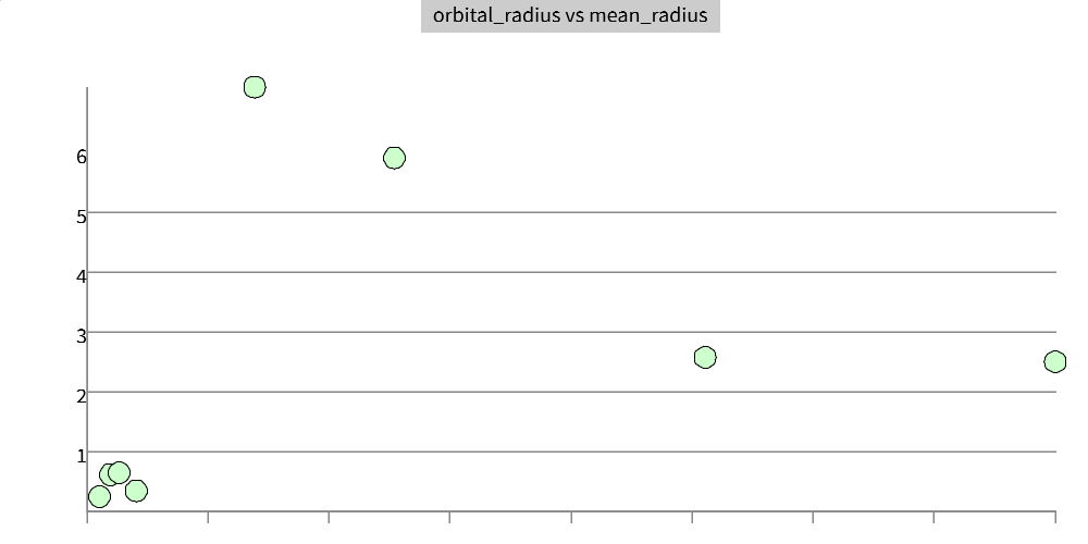
Now let's compare the radius of the orbit to the radius of the planet. This will show us if the smaller planets are clustered together or spread out.
planets << dataset("planets") chart(planets, type : "scatter", x : "orbital_radius", y : "mean_radius")
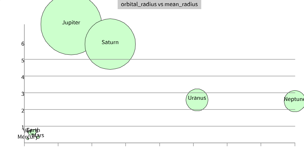
Now lets make the size of the circle represent the size of the planet and show the names
planets << dataset("planets") chart(planets, type : "scatter", x : "orbital_radius", y : "mean_radius", size : "mean_radius", name : "name")
Here's a fun one. Let's see which letters have one syllable vs two.
//TODO: this is broken when doing builddocs chart(dataset('letters'), y_value:'syllables')
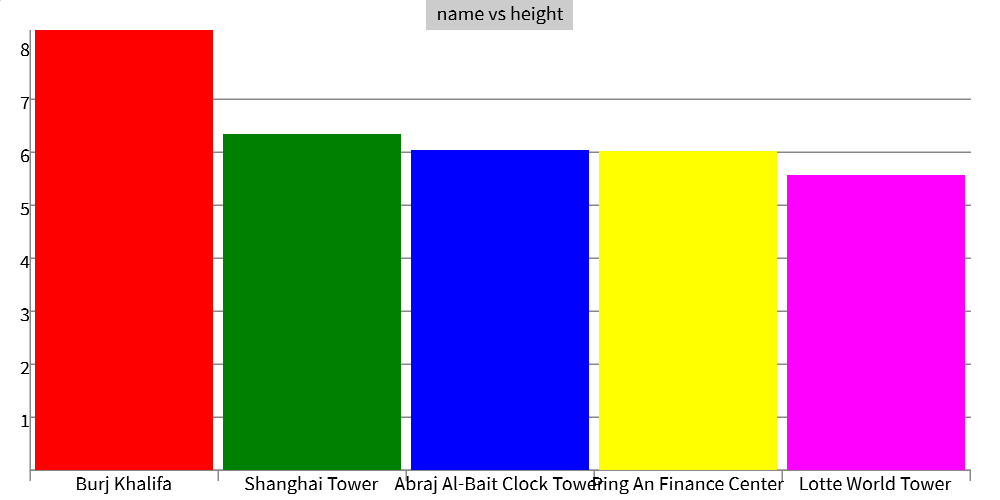
Let's check out the relative heights of the tallest buildings in the world:
buildings << dataset("tallest_buildings") b2 << take(buildings, 5) chart(b2, y : "height", x : "name")
Histograms
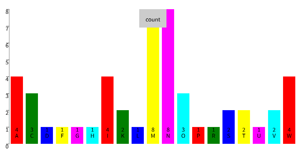
states << dataset("states") first_letter << (state : ?)->{take(get_field(state, "name"), 1)} states << map(states, first_letter) histogram(states)
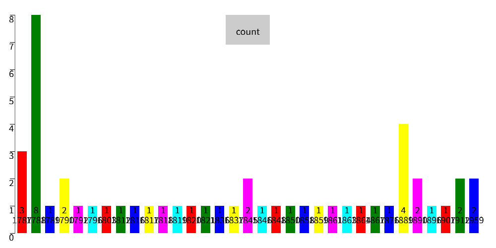
Statehood date by year by decade
states << dataset("states") get_year << state-> field << get_field(state, "statehood_date") dt << date(field, format : "MMMM dd, yyyy") get_field(dt, "year") years << map(states, with : get_year) histogram(years, bucket : 10)
Random Numbers
Filament can generate random numbers for you. Now you might wonder why this is useful. It turns out random numnbers are incredibly useful for all sorts of things, from drawing graphics to simulations, and of course they are heavily used in video games.
To make a random number just call random
random()
0.568
Every time you run this function it will return a different number.
By default the number will always be between 0 and 1, but you can choose a different max and min if you want.
Suppose you want twenty random numbers between 5 and 10 you could do this:
range(20) >> map(with : n->random(min : 5, max : 10))
8.416, 5.059, 6.922, 9.190, 8.431, 5.786, 8.621, 8.192, 5.903, 5.280, 5.415, 6.291, 5.616, 8.128, 5.377, 5.691, 9.626, 6.747, 7.131, 5.057
Mapping a range is an easy way to create a list, then call random on each one to make the final numbers.
However, making lists random numbers is so common you can just call random directly using count .
random(min : 5, max : 10, count : 20)
6.921, 8.424, 8.157, 9.260, 6.057, 7.271, 5.732, 7.119, 9.913, 8.501, 9.278, 9.445, 5.478, 7.077, 9.210, 7.632, 5.488, 5.918, 9.123, 8.844
Making Shapes
Filament makes it easy to draw shapes. Let's start with some simple squares.
Drawing Squares
To create a square call the rect function with a width and height, then
send it into the draw() function to show up on the screen.
rect(width : 100, height : 100) >> draw()

By default the shape is the upper left, but you can change the x and y to put it wherever you want.
rect(x : 200, y : 100, width : 100, height : 100) >> draw()

If you want to draw more than one shape, just put them into a list. You can even use units for the size of your shapes. Below are two rectangles, one in centimeters and one in inches. If you don't include any unit then Filament assumes it is in pixels.
[rect(x : 0, width : 1cm, height : 5cm),rect(x : 50, width : 1in, height : 1in)] >> draw()

Along with size, you can also set the color of shapes using
the fill argument. You can set it to named colors as strings like
"red" , "green" , and "green" or use a list of three numbers
between 0 and 1. These will be interpreted as RGB values.
so
rect(width : 10cm, height : 10cm, fill : "blue") >> draw()

is the same as
rect(width : 10cm, height : 10cm, fill : [0,0,1]) >> draw()

You can draw multiple shapes by putting them
into a list, but then they might draw on top of each other
unless you manually set their x,y positions. Since it's
common to want to put shapes next to each other, you can
use the row function to space them out, with an optional
gap parameter
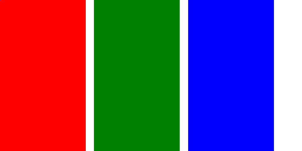
[rect(width : 10cm, height : 20cm, fill : "red"),rect(width : 10cm, height : 20cm, fill : "green"),rect(width : 10cm, height : 20cm, fill : "blue")] >> row(gap : 1cm) >> draw()
Can you guess what column does? :)
This means you could make your own bar chart from scratch!
range(5) >> map(with : n->rect(width : 1cm, height : n * 5cm)) >> row(valign : "bottom", halign : "center") >> draw()

Other Shapes
circle
circle(x : 4cm, y : 4cm, radius : 2cm, fill : "aqua") >> draw()

making art
Make some cool artwork with random numbers
make << (n)->{ rect(x : random() * 200, y : random() * 200, width : 100, height : 100, fill : [n / 100,random(),0]) } range(100) >> map(with : make) >> draw()
Random Colors
Now let's use it to make some random colors. First I want to give Martin Ankerl credit for his original article on making pretty random colors. Thanks Martin.
In Filament, colors are made using a list of three numbers, each from 0 to 1. They represent the
red, green, and blue (RGB) parts of the color. Thus [0,1,0] would be pure green and [1,1,1] is
pure white.
Let's make 20 randomly colored squares.
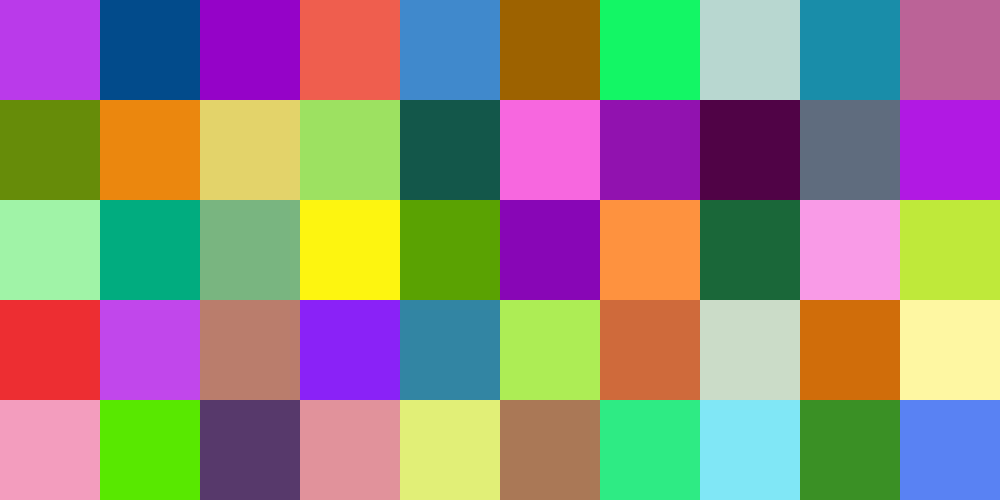
make_square << ()->{ rect(width : 100, height : 100, fill : [random(),random(),random()]) } range(50) >> map(with : make_square) >> row(gap : 0) >> draw()
Hmm. Those are pretty ugly. Some colors are too dark. Some are too similar. The problem is that we are using the RGB color space . We don't have a way to make the colors more similar easily. However, there is another color space we can use called HSL for Hue, Saturation, and Lightness. This way we can have a single number for the hue (the 'color'), and keep the saturation and lightness fixed. Then we can convert them back to RGB to draw them.
For the conversion we have a handy function called HSL_TO_RGB function. It takes the hue,
saturation, and lightness the 0-1 range, returns RGB in then 0-1 range.
make_square << ()->{ color << [random(),0.8,0.9] rect(width : 100, height : 100, fill : HSL_TO_RGB(color)) } range(50) >> map(with : make_square) >> row(gap : 0) >> draw()
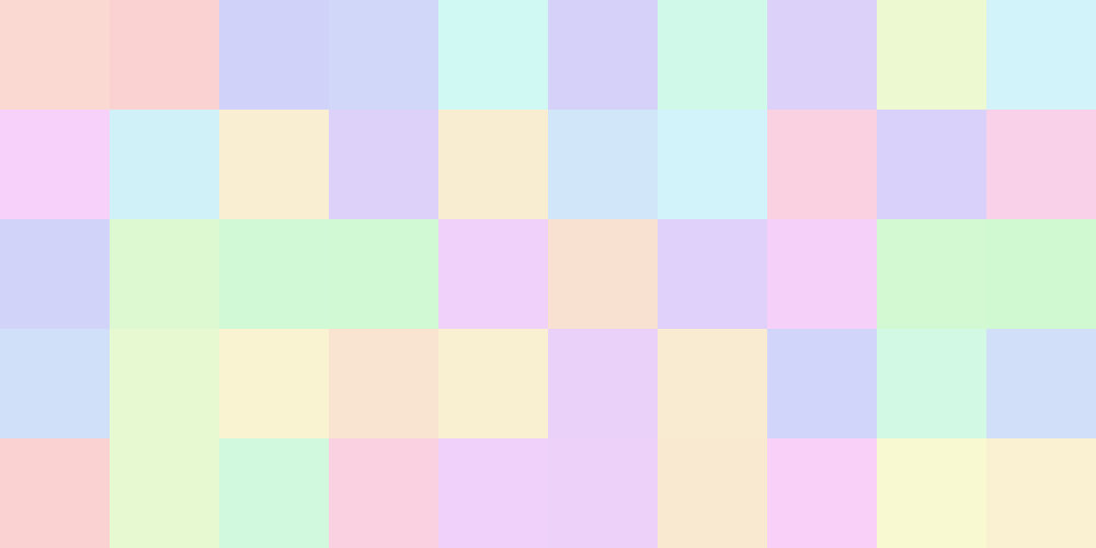
In the code above we choose a random hue but keep the saturation at 0.8 (sort of pastel like) and the lightness almost at 100%.
Let's try that again with different S and L values. Lower the saturation to 0.5, meaning it's partly gray, and move lightness to 50% (0.5)
make_square << ()->{ color << [random(),0.5,0.5] rect(width : 100, height : 100, fill : HSL_TO_RGB(color)) } range(50) >> map(with : make_square) >> row(gap : 0) >> draw()
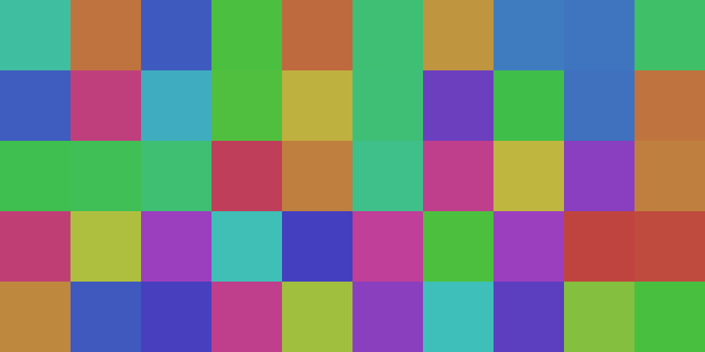
These look better. Each color is the same distance from black and white, so we are getting some nice hues. However, it's still pretty random. You'll notice that sometimes the colors clump together. Instead we'd like to have them distributed evenly across the hue.
There's a clever trick we can use with the golden ratio. Start with a random number then add the golden ratio (1.618) to it. Each time we wrap it back around at 1. This works because the hue is like a circle. When you go far enough to the right edge it wraps back around. Thanks to the golden ratio it will keep looping around and always pick a new hue value distant from the previous ones.
Note that I'm using the Golden Ratio Conjugate, which is the reciprical of the Golden Ratio. Also note that Filament doesn't have loops yet, so I'm using a recursive version.
GRC << 0.618033988749895 make_square << (depth,h)->{ color << [h,0.5,0.5] ifdepth <=0 then rect(width : 100, height : 100, fill : HSL_TO_RGB(color)) else [rect(width : 100, height : 100, fill : HSL_TO_RGB(color)),make_square(depth - 1, h + GRC)] } make_square(50, random()) >> row(gap : 0) >> draw()
There we go. That looks great! Why don't you try it yourself and change the saturation and lightness values.
Images
New Images from Scratch
Filament can create images with colors, just like shapes. The difference is that an image is made of pixels and you must specify a width and height.
make_image(width : 100, height : 100) >> map_image(with : (x,y)->{ [1,0,0] })

The code above creates an image filled with rect. The map_image calls
the function you pass to it for every pixel. This function should return a new
color for that pixel. Colors are represented as RGB, in the range 0 to 1, just
like with shapes.
This means red << [1,0,0] , blue << [0,0,1] , and gray << [0.5,0.5,0.5] or [50%, 50%, 50%]
Let's make another image where instead of using a single color, we calculate a new random grayscale value for each pixel.
make_image(width : 100, height : 100) >> map_image(with : (x,y,color)->{ n << random(min : 0, max : 1) [n,n,n] })
So far we have ignored the x and y values, but if we use them we can create patterns that vary over space. Let's make stripes where teh color changes based on if the x value is even or odd.
red << [1,0,0] green << [0,1,0] make_image(width : 100, height : 100) >> map_image(with : (x,y,color)->{ ifx mod2 =0 then red else green })

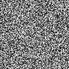
We can even draw shapes pixel by pixel using implict equations. For example if let's calculate the distance of a pixel from the origin. If it's greater than some threshold then make it be red, otherwise green. This is similar to how GPU pixel shaders work.
dist << (x,y)->{sqrt(x ** 2 + y ** 2)} make_image(width : 100, height : 100) >> map_image(with : (x,y,c)->{ ifdist(x, y) <100 then[0,1,0]else[1,0,0] })
Loading Images from the Web
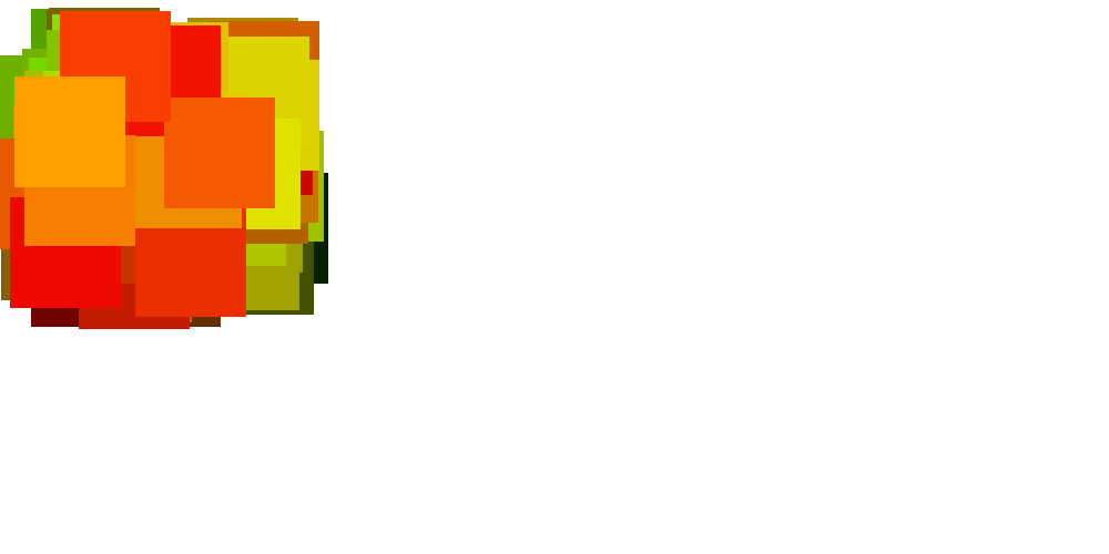
We can load an image from the web using the load_image function.
filament
load_image(src:'https://vr.josh.earth/webxr-experiments/nonogram/thumb.png')
Once we have the image we can modify it. Let's drop the red channel by returning a new color that only includes the green and blue values from the original pixels.
load_image(src : "https://vr.josh.earth/webxr-experiments/nonogram/thumb.png") >> mapimage(with : (x,y,c)->{ v1 << 0 v2 << (c[1]) v3 << (c[2]) [v1,v2,v3] })
We can also make an image grayscale by averaging the colors.
load_image(src : "https://vr.josh.earth/webxr-experiments/nonogram/thumb.png") >> mapimage(with : (x,y,c)->{ n << sum(c) / 3 [n,n,n] })
Converting to grayscale by averaging the red green and blue does work, but it doesn't loook very good. Taht's because it doesn't acocunt for the fact that the human eye is more sensitive to blue than to green or red. Let's create a few functions to make it work better.
first we need brightness base on a more accurate grayscale conversion
brightness << (c)->{c[0] * 0.299 + c[1] * 0.587 + c[2] * 0.114}
UNKNOWN
Now let's create a function to mix two colors together using a t value that goes from 0 to one. If t is 0 then you get only the first color. If it's 1 then you get only the second color. Otherwise you get a mixture of hte two. Sometimes this is called a lerp function, short for interpolate.
mix << (t,a,b)->{a * t + b * (1 - t)}
UNKNOWN
Now that we can mix two colors, we can use black and white for grayscale. But we could also use white and brown for a sepia town, or even something crazier like red and blue.
brightness << (c)->{c[0] * 0.299 + c[1] * 0.587 + c[2] * 0.114} mix << (t,a,b)->{a * t + b * (1 - t)} white << [1,1,1] brown << [0.5,0.4,0.1] sepia << (x,y,color)->{ brightness(color) >> mix(white, brown) } load_image(src : "https://vr.josh.earth/webxr-experiments/nonogram/thumb.png") >> mapimage(with : sepia)
brightness << (c)->{c[0] * 0.299 + c[1] * 0.587 + c[2] * 0.114} mix << (t,a,b)->{a * t + b * (1 - t)} red << [1,0,0] blue << [0,0,1] rb << (x,y,color)->{ brightness(color) >> mix(red, blue) } load_image(src : "https://vr.josh.earth/webxr-experiments/nonogram/thumb.png") >> mapimage(with : rb)
Turtle Graphics
Based on this tutorial. link
Turtle graphics is a different way of generating images than setting pixels or drawing shapes on the cartesian plane. Instead of saying "put a shape here", you have a turtle with a pen which draws the shapes for you. I know that sounds confusing, so let's start with some examples.
How Turtles Move
Image a turtle walking around in an infinite plane. Starts at the center and is pointed north. You can tell turtle to move forward or to turn. to start, let's tell it to move forward by 100 pixels.
turtle_start(0, 0, 0) turtle_pendown() turtle_forward(100) turtle_done()

Now let's tell it to turn right and move forward another hundred.
turtle_start(0, 0, 0) turtle_pendown() turtle_forward(100) turtle_right(90) turtle_forward(100) turtle_done()
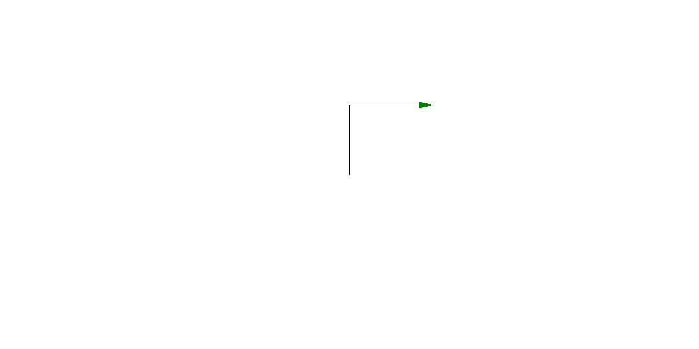
Now we have an L shape. The turtle is carrying a pen, so every where it moves it draws a line.
Now let's make a square by doing it four times.
turtle_start(0, 0, 0) turtle_forward(100) turtle_right(90) turtle_forward(100) turtle_right(90) turtle_forward(100) turtle_right(90) turtle_forward(100) turtle_right(90) turtle_done()

Now we have a square. Of course, writing 'right' 'forward' over and over is annoying. Instead let's use a loop to do it four times.
turtle_start(0, 0, 0) range(4) >> map(with : ()->{ turtle_forward(100) turtle_right(90) }) turtle_done()

Much better.
Shapes
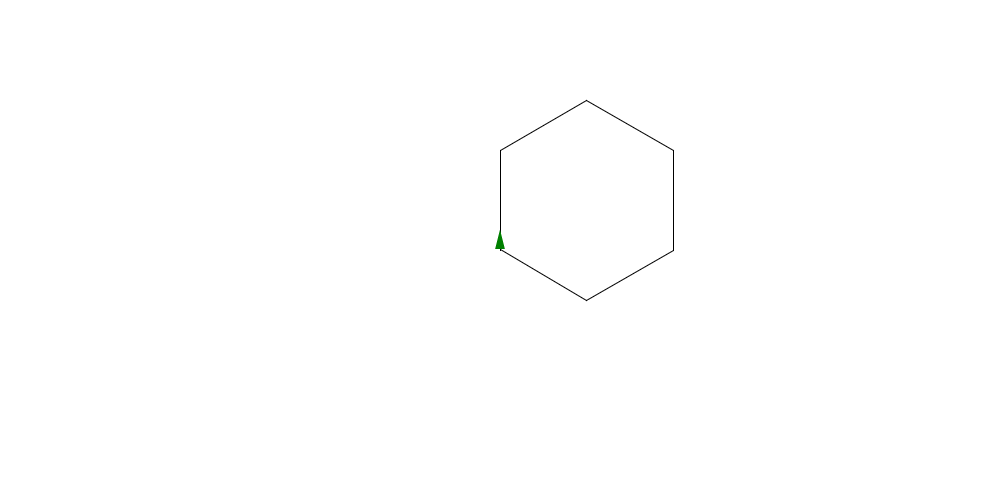
Now that we know how to make a square, we can clearly see how to draw a hexagon. Loop 6 times and turn right by 60 degrees
turtle_start(0, 0, 0) range(6) >> map(with : ()->{ turtle_forward(100) turtle_right(60) }) turtle_done()
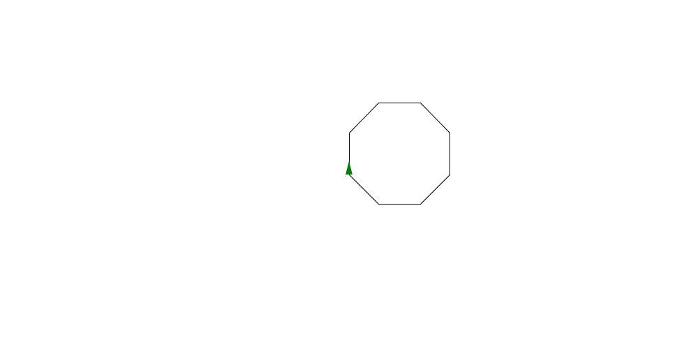
We can start to see a pattern. For any regular polygon with N sides we loop N times and turn by 360/N. Let's make some code to draw any sort of polygon. We can change the value of N to draw a different shape. Here it is for an octogon.
turtle_start(0, 0, 0) ngon << (N,side)->{ range(N) >> map(with : ()->{ turtle_forward(side) turtle_right(360 / N) }) } ngon(8, 60) turtle_done()
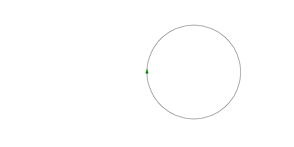
If we change N to 100 and size to 10 it looks like a circle.
turtle_start(0, 0, 0) ngon << (N,side)->{ range(N) >> map(with : ()->{ turtle_forward(side) turtle_right(360 / N) }) } ngon(100, 10) turtle_done()
Colors
What's even cooler than drawing a shape from lines, is drawing a shape over and over. Let's go back to drawing a square, but do it over and over with a slight rotation.
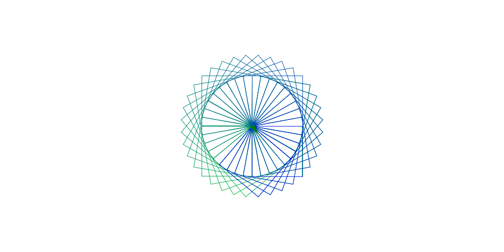
turtle_start(0, 0, 0) ngon << (N,side)->{ range(N) >> map(with : ()->{ turtle_forward(side) turtle_right(360 / N) }) } range(50) >> map(with : ()->{ ngon(4, 100) turtle_right(10) }) turtle_done()
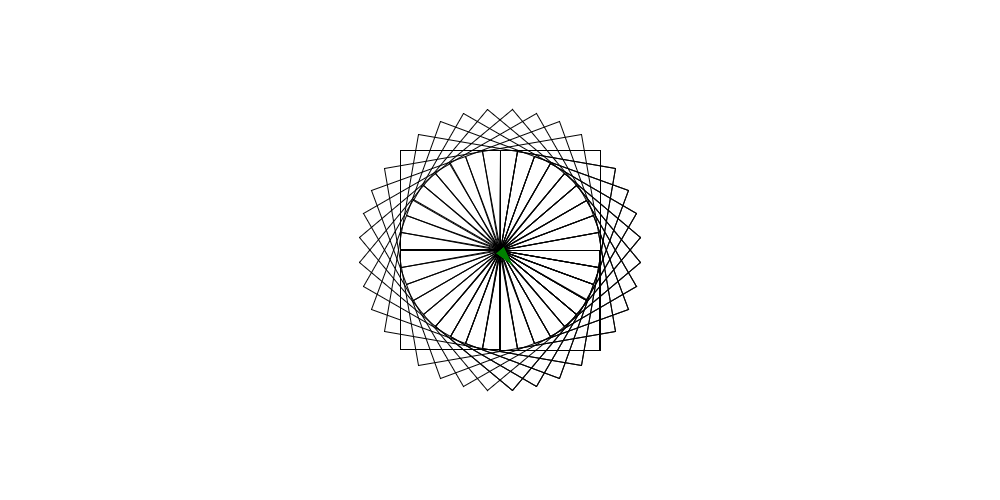
Woah!
Now let's switch colors each time with turtle_pencolor()
turtle_start(0, 0, 0) ngon << (N,side)->{ range(N) >> map(with : ()->{ turtle_forward(side) turtle_right(360 / N) }) } range(50) >> map(with : (i)->{ ngon(4, 100) turtle_right(10) t << (i / 50) turtle_pencolor([0,1 - t,t]) }) turtle_done()
Turtle graphics is a really fun way to draw shapes incrementally. What we've done is define a small thing, a side, then repeat it to make a shape, then repeat that to make a more complex shape.
Complex Shapes
For our final example let's draw a flower. How could we do this? Why don't we start with a petal, figure that out, then draw it a bunch of times to make the flower. But how do we draw a petal? By breaking it down into even smaller pieces.
We learned to draw a curve by doing lots of short lines. Let's do just a partial circle.
turtle_start(0, 0, 0) arc << ()->{ map(range(120), with : (n)->{ turtle_forward(2) turtle_right(1) }) } arc() turtle_done()
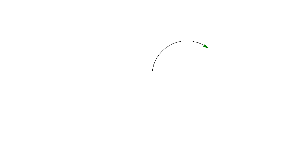
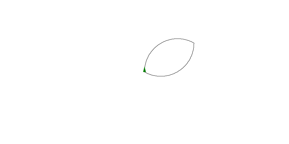
Perfect. Now we can rotate and do it again
turtle_start(0, 0, 0) turtle_pendown() arc << ()->{ map(range(120), with : (n)->{ turtle_forward(2) turtle_right(1) }) } leaf << ()->{ arc() turtle_right(60) arc() turtle_right(60) } leaf() turtle_done()
Now we have a full petal. To get a complete flower we just need to do it a bunch of times.
turtle_start(0, 0, 0) turtle_pendown() arc << ()->{ map(range(120), with : (n)->{ turtle_forward(2) turtle_right(1) }) } leaf << ()->{ arc() turtle_right(60) arc() turtle_right(60) } range(36) >> map(with : ()->{ leaf() turtle_right(10) }) turtle_penup() turtle_done()
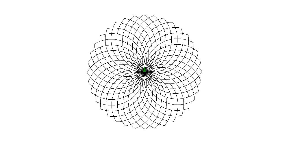
Now we have a complete flower. Most programming is like this. We build big complex things out of lots of smaller, simpler pieces.